25-March-2015: Centripetal Acceleration vs. Angular Frequency

Purpose: We will be exploring the relationship between centripetal acceleration and angular speed.

Allow me to define angular frequency, angular speed, and centripetal acceleration. 
Angular frequency (ω) is a scalar measure of rotation rate. It refers to the angular displacement per unit time or the rate of change of the phase of a sinusoidal waveform, or as the rate of change of the argument of the sine function. Angular speed is the rate at which an object changes its angle, measured in radians, in a given time period. Angular speed has a magnitude (a value) only. 

Centripetal acceleration is the rate of change of tangential velocity.

For our experiment we will be sharing data with the class. Due to the lack of equipment available for each group our professor ran a series of trials in which we recorded the initial time (one rotation), final time (ten rotations), and acceleration in the x axis.

If we were to do it on our own, our apparatus for this experiment would look like the above picture. There is an accelerometer on the disk with tape sticking out to the photogate. The wheel on the left is powered by a battery source and will turn the disk at a desired voltage. We took our measurements at six different voltages; 4.8, 6.2, 7.8, 8.8, 10.8, and 12.6. Each one we recorded the initial time (one rotation), final time (ten rotations), and acceleration in the x axis.

Above image: We obtained our initial and final time from these recordings.

Above image: Minus the 6.2 volts, we had the rest on one chart. Using the mean gave us a value for acceleration.


We then took the data we gather and recorded them onto excel. Using excel's calculation capabilities we input the formula for ω. Refer to the top for the equation of ω, where 2*pi is in radians and time is for one rotation.

We then plotted an acceleration vs. angular speed^2 graph. The slope gives us the radius in meters.

Conclusion

The slope in our graph above tells us the distance from center and end point of the disk. We were able to use acceleration and angular speed to find a general length of our circle. Theory predicts that if either our acceleration or angular speed were to increase or decrease, so would the radius of the disk. Essential by using the relationship of these two we can determine the size of any circular disk.

Errors that may pertain to this experiment could be the equipment. The photogate is old and the tape that it is suppose to read can give an error. The equipment was taped onto the disk. Knowing that, as the disk spins faster and faster whose to tell that the equipment may or may not have slipped from its original position. We noted that the initial time was not making sense at first, but came to realize that the tape passing through the photogate started at different positions. That is why we took the time at ten rotations and divided it by ten for an average. Even ten may not have been enough, with more rotations, say 50, would have possibly provided a better value.

23-March-2015: Trajectories

Purpose: We are going to utilize our understanding of projectile motion to predict where a ball rolling down a ramp will land on an inclined board.

There will be two parts to this experiment. First we will construct an apparatus that will allow us to roll a ball down a ramp and off the table.

Once our apparatus was built. We rolled the ball to see where it would land so that we may lay down carbon paper to help keep track of the landing. We rolled the ball from the same place five times down the ramp and each time the ball landed on the carbon paper it left a mark that we will use to take measurements.

The data we will use is the length in the horizontal and vertical direction from which the ball leaves the ramp. The vertical length does not change and we recorded 0.96 m. The horizontal length we gathered a range from launching the ball five times from the same place, 0.765 m to 0.785 m.

With length in both the y and x direction we used kinematic equations to calculate the time in which the ball will land on the ground when leaving the table. Using that same time we calculated the initial velocity from which the ball leaves the table.

Time it took to hit the ground 0.443 s.
The initial velocity in the x direction is 1.75 m/s.
Note that the initial velocity in the y direction is zero because at the moment the ball leaves the ramp the only momentum propelling the ball forward is all in the x direction.


Second part of this experiment is where a wooden board will be leaning at the edge of the table. Keeping in mind that the wooden board will be as close the edge of the ramp not allowing any extra length from which the ball leaves the ramp.

Launching the ball from the same spot as the first part. We will be deriving an expression that will allow us to determine the value of "d". We know our initial velocity from before and another key data to record is the angle the board is from the horizontal. Using the phone application the can measure angles we recorded our angle to be 49 degrees.

Now we derived our expression as so.

Using kinematics we will be combining the x and y and rearrange in terms of d.

Again with our initial velocity and angle we were able to calculate where the ball should land on the board. Our calculated distance was 1.0959 m.

Now we rolled the ball down the ramp onto the carbon paper tapped onto the wooden board five times. This gave us a range we measured 0.98 m  to 1.015 m.

As you can see our calculated value for the distance was slightly larger than what we measured from the carbon paper.

We will now use propagation to find if our uncertainty of distance that will help out our calculated value with the measured values. Our uncertainty for measuring the distance in the x and y direction is +/- 0.02 m. The uncertainty for the angle was +/- 0.0017 in radians.

Before we can get to propagating an uncertainty we need to create an expression that will give us values for x, y and the angle.

Once we found a suitable expression we can use. We found our uncertainty.

Conclusion

Putting it all together our calculated distance with the uncertainty was.

1.0959 m +/- 0.086 m

Now comparing it to the measured values. We calculated where our ball would land within the ranges and we were successful in meeting with the measured values.

Granted we were a bit on the higher end of the values. That could be interrupted by error from either how much gap there may have actually been between the wooden board and the ramp from which the ball leaves the table. People were walking around our table on which our apparatus was on and may have bumped it causing it to move. It is also possible that the wooden block slid.

18-March-2015 Modeling Friction Forces

Purpose- This lab is a series of five different experiments that we will be conducting to obtain a targeted variable, revolving around the coefficient of static and kinetic friction. In the last experiment we will use kinetic friction to predict an acceleration of an object.



Experiment One - Static Friction

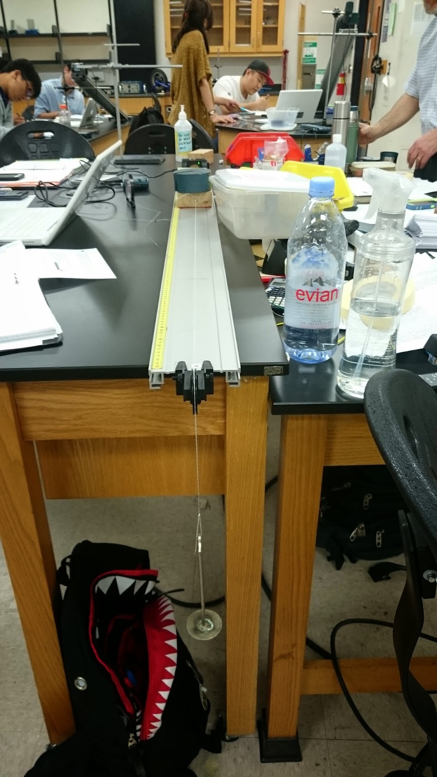
Static friction is a force that is between two objects when they are not moving. In our first experiment we are going to set up a pulley system with a block on a horizontal plane and a cup hanging from the pulley. Both the block and cup are attached to each other keeping in mind that the string is leveled horizontally to the plane of the tabletop.

To find our maximum static friction. We will be adding water into the cup until the block begins to slide. When the block slides we remove just enough water so that the block remains in equilibrium.

We repeat this process by stacking an additional block till we have a total of four blocks stacked.

Data we recorded were the mass of each block and total mass of the cup filled with water.

Note: units are in grams

We then developed a free body diagram to determine our forces for the block and the cup.

Using the technique we can break our net forces of each object into a force in the x direction and force in the y direction. 

F=ma but in this case with nothing moving we can say our acceleration is zero. 

Block forces in the x direction ends up becoming : T - friction = 0

Block forces in the y direction ends up becoming : N - Mg = 0

Cup forces in the x direction has none.

Cup in the y direction has :                                      mg - T = 0

Essential for this scenario our normal force equals the weight of the block and our friction force equals weight of the cup. 

We will input our data and formulas into logger pro to develop a static friction force vs. normal force graph. The graph then requires a proportional fit so that our slope (A) gives us the coefficient of static friction.

Coefficient of static friction = 0.2844




Experiment Two - Kinetic Friction

Kinetic friction is the sliding force between two objects. The force is always opposite from the direction of motion, is proportional to the normal force, and independent of the area or speed of the moving object.

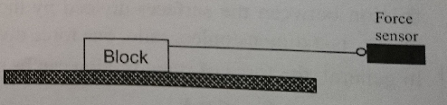
For the second experiment we will be attaching a force sensor to a block(s), keeping in mind to keep the string leveled to the horizontal plane.

 

 We are using the same blocks that we found our coefficient for static friction with. Calibration is in order for the force sensor to work properly. As we collect data we are pulling the block at a constant speed and allowing logger pro to work its magic. We repeat this until we have four blocks stacked.

Image below: Thinking about why the force from each collected data was slightly higher. The reason being is that with an additional block added each trial, the force required to pull the block increased.
Instead of plotting for a slope this time we took the mean from each trial. Keeping in mind to choose a range that best represented a good data at constant speed.

We then took our data and recorded it into a fresh sheet. Using logger pro to develop a kinetic friction force vs. normal force graph. (Normal force is obtained the same method as from the static free body diagram : N=Mg) The slope here gave us our value for the coefficient of kinetic friction.

Coefficient of kinetic friction = 0.2767




Before we move onto the next experiment lets think about our values of coefficients for static and kinetic friction.

Coefficient of static friction = 0.2844
Coefficient of kinetic friction = 0.2767

Does it make sense that our coefficient of static friction is higher than our coefficient of kinetic friction?

Yes is does. Generally speaking to maintain an object at rest would require a bit more force to remain still.
Also because everything on the internet is true, refer to the image below.

Experiment Three - Static Friction From A Sloped Surface


In this experiment we will be testing the blocks capability to remain still on an angled surface.

We begin by placing a block on a horizontal platform. Then we raise the platform just until the block begins to slide down. This will give us a good idea of the coefficient of static friction between the block and the surface.
Once we found the max incline at which the block will remain in equilibrium. We measured the angle between the platform and the table.

Our angle was 15 degrees.
Mass of the block 0.1217 kg.

We drew a free body diagram that modeled the block at its incline. Solving for the coefficient of static friction calculated to equal tan(theta).

Coefficient of static friction equaled 0.2679.



Experiment Four - Kinetic Friction From Sliding A Block Down An Incline


This experiment is similar to the third one. Our hopes here, is to determine the coefficient of kinetic friction as the block slides down the incline.

We will use the same set up as the third experiment but this time have a motion detector at the top of the incline. As we collect data, logger pro will use the motion detector to collect the velocity at which the block slides down and its time interval.

Setting up our velocity vs. time graph in logger pro. We fitted our line to give us a slope which will tell us our acceleration.

Acceleration = 0.1725 m/s/s
Mass of the block = 0.1217 kg
Angle = 17 degrees

This time we have a motion going down which allows F=ma for our net force in the x-direction to keep "ma". Where as in the static portion, since our system was in equilibrium, the acceleration was zero.

For this experiment we solved for coefficient of kinetic friction it ended up equaling
tan(theta) - a / g * cos(theta)

Using this our value yielded 0.287.

Experiment Five - Predicting The Acceleration Of A Two-Mass System


Finally we are going to derive an expression that will predict the acceleration of our sliding block.

In this system we have the same motion sensor on one side and a pulley with a hanging mass. The hanging mass is heavy enough, that when left to nature, will slide the block across the horizontal surface.

Before we run anything through logger pro we will calculate ourselves what we hope the acceleration will be. We will be using the coefficient of kinetic friction we gathered from experiment four, the mass of the block and the hanging object. Deriving an expression for acceleration, we will plug in those values to obtain our acceleration.

We calculated out acceleration to be 0.93768 m/s/s

Next we ran our system through logger pro. Logger pro developed for us a velocity vs. time graph. Fitting the line we found the slope (acceleration) to be 0.8137 m/s/s

Calculated acceleration 0.93768 m/s/s
Logger pro acceleration 0.8137 m/s/s



We have a conflict in values for acceleration. Its about a ten percent difference. Errors and determining values are cause by many things. First issue that we have to take into consideration is the equipment we had available to us. These devices we use to measure our systems are old and cheap. They provide a decent range of certainty but they go so far. If we needed more precise means to measure our system components individually and during motion. As students we would need to have high priced tools that measures more precisely. Being that we are not equipped for it. Having an error ten percent within our values is close enough.

Mainly to take away from these experiments is preservation of knowledge in the steps we used to obtain our targeted values. Which in this case was mainly revolving around the coefficients of static and kinetic friction.

11-March-2015: Modeling the fall of an object falling with air resistance

Purpose - We will be able to obtain a relationship between air resistance force and speed. Once a relationship is found we will be using excel to predict the terminal velocity and compare the values.

Part 1 
In this part we will be taking coffee filters and dropping them so that we may develop our terminal velocity by allowing the computers camera to record the time and distance the filter falls. We are going to repeat this process five times each time adding another coffee filter. Once all five videos are recorded we will use logger pro to measure our position and time by placing dots in each video as the filter falls.

Image on right: This is our experimental ground. You see we have to identify a marker so that we can give logger pro a set of data in which to measure the distance in which the coffee filters will fall. Once the marker was established we proceeded to drop the coffee filters as logger pros video function captured each fall.

We repeated dropping the coffee filter five times. Each time adding a coffee filter stacked on one another.

Image below: To obtain position vs. time graph we plotted dots on each time frame in the videos we captured. We followed the coffee filters drop adding each dot to each frame while logger pro calculating the data we needed. Once we dotted each frame and had enough data to work with. We highlighted a good range on the graph from which we will achieve a value for terminal velocity (which is the slope) with respect to the amount of coffee filters we had stacked.

Note: Pay close attention to the slope given. It is negative for all five we fitted but we will end up taking the absolute value of each slope.



We have an expectation that air resistance force on a particular object depends on the object's speed, shape, and the material it is moving through this equation.

To find our value of k and n. We are going to have to calculate a couple things and plot it on to logger pro. Logger pro is great at making graphs and giving out information in which we will translate to finding our k and n.




Image Below: We have a free body diagram of how our coffee filter is while falling. Lets say our downward motion is positive and knowing that our speed is constant. Net F=ma in the y-direction. We have F=mg. We know mass from weighing them and gravity we use 9.8 m/s/s. We calculate our force.

Image below:  Obtaining our terminal velocity and force. We record the data into logger pro which displays a nice graph in which to find k and n. In this case A=k and B=n.

Part 2
We will be developing a mathematical model on excel. The goal is that we will be able to predict the terminal velocity of 1 or more coffee filters.

Image below: For excel we need to formulate an equation for acceleration involving our air resistance force. Notice in the boxed area we find how we will be plugging in an equation for our acceleration into excel.

In excel we will set in our first 5 rows in column A the values our obtain from our calculations. Mass and our time interval will vary. Mass varies by deciding whether it is one filter or five filters we can sum the mass and plot into excel. Time interval varies by how we can view our value shorter in range.

Note: I kept highlighted the box we input our equation of acceleration into.

Once we plotted the necessary data onto excel. We dragged down the columns and allowed excel to calculate the prediction for terminal velocity. 

We know terminal velocity occurs when acceleration reaches zero. Image Above: In purple is acceleration reaching zero and in red is velocity. If you remember from the first graph we obtain from logger pro the numbers are very close to one another.


Image Below: This is a velocity vs. time graph. Notice as time passes our object begins to level off and our velocity is becoming constant. Which give us a max value.

Conclusion

We ultimately learned two ways in which we are able to calculate terminal velocity. First method was through logger pro and its nice video function. Logger pro gave us slopes that meant terminal velocity. We derived a function to use into our acceleration column in excel. Plotted data and knowing that when acceleration reaches zero we have terminal velocity.

With logger pro we had some obstacles that may have infringed on certain values. For example, while plotting dots in the video frames. Visually finding where our coffee filter was a challenge at times. Which may have lead to some error in how logger pro calculates. 

The model in excel gave us a more precise value in terms of our calculation we entered. Any error from excel would have been from the measuring devices for mass of our coffee filter (which effect logger pro as well). Generally most the values we obtained were from logger pro. If any error may have been presence it all began from logger pro.

In the end comparing our values for terminal velocity in logger pro and excel were close enough to validate that both warrant sufficient enough values. 

09-March-2015: Propagated uncertainty in measurements

Part 1 - Measuring the Density of Metal Cylinders

Purpose - We will be introduced to propagating uncertainties in the measurements we take for our data which leads to uncertainty in the final result. This simply means that we are going to find a range of values that will be with-in the accepted value. For instance, if we take a pen and weigh it on a scale. The scale is a cheap one so the range of uncertainty on the weight of the pen will be +/- the value on the display of the scale. 

Step 1 - For this lab we are given three different size metal cylinders. With a scale and caliper we are to measure the weight, diameter and length of these three objects. 

As you can see highlighted we have the value the scale displays, in blue. Something to note is in red. That is the uncertainty value +/- 0.1 grams from the measuring tool. Which we will need later.

Image Below: Here we have a caliper that will measure the length and diameter of the metal cylinder. As you can see it is pretty difficult to read the value. Notice the blue arrow points to the tick mark that we will use to record the data. If you look closely the tick mark is between the 1.2 cm and 1.3 cm. To record our data we use an educated assumption that the value the caliper is providing us with, is a diameter of 1.24 cm.

Image Below: This is our data table we collected from measuring all three metal cylinders with the tools mentioned above. Note that with the size difference, some how the masses are identical to the tenth decimal place.
If we think about the different densities of metal in the world. We can assume that lead is denser than iron and iron denser than aluminum. Given our type of metal cylinders we know that we can find an actual value that we can compare with our record data. Doing so will brighten our insight on how uncertainties in each measurements will effect our final recorded value.

Note that height, diameter and mass we recorded has an uncertainty. As we find densities for each metal cylinders they too will have an uncertainty from the measurements written.

Step 2 - The data we record will assist in determining the densities of these three objects.

Image on right explains the density formula.









If you notice the data we recorded is missing volume. Therefore, we are going to use another formula that will give us our volume.

Image below gives us an understanding on how we will find our volume. 

pi is 3.14...
r is radius which is half of a diameter
h is height

If we combine the volume formula into the density formula we will obtain a means to calculate our density with the information we have.

Substituting volume of a cylinder into our density formula will give us the densities we require.

Step 3 - Propagating the uncertainties of each measurement.

To propagate an uncertainty in the measurements we will use a calculus technique called partial derivatives. It follows some of the same principals as deriving equations. Instead of traditionally taking a number and variable and deriving. We will use our formula of density that we substituted the volume of a cylinder into.

Note we have three variables; m for mass, d for diameter, and h for height.

We will take each variable and partially derive each of them. Each variable we partial derive will also be multiplied by the uncertainty from the measuring tool. We accomplish partial derivative by taking which ever variable we will partial derive, derive that and treat everything else as constants.

For example, if our mass was the variable we are partially deriving. The diameter and height variables would act as a constant and as I would say "move to the front of the bus." No need to do that power stuff like bring the n down and subtracting n by one afterwards. That only applies to our mass variable.
Same goes if diameter was our variable we are partially deriving. Mass and height would be the constants.

If height is the variable were partially deriving. Mass and diameter would be constants.

Note that the funny looking d is the symbol to describe partial derivatives.

Once we get our values from partially deriving each variable we will absolute each value and sum them all up. That value then becomes our uncertainty for density of which ever metal cylinder is plugged in.

Below Image: This is a sample of how we calculated one of our metal cylinders.

Our calculated results

Density for lead and uncertainty:               11.55  g·cm⁻³  +/- 0.2808  g·cm⁻³
                                                                   

Density for iron and uncertainty:               6.72  g·cm⁻³   +/- 0.3314  g·cm⁻³

                                                                 

Density for aluminum and uncertainty:     2.427  g·cm⁻³ +/- 0.0463  g·cm⁻³

                                                                   

Accepted values

Density for lead:                                        11.34 g·cm⁻³

Density for iron:                                        7.874 g·cm⁻³

Density for aluminum:                              2.70 g·cm⁻³

Conclusion - Comparing both our calculated results and the accepted values we find that both are marginally close. Iron for us was probably the furthest away from the accepted value. Which could either mean the measuring tools were that old or some where along the way we made a mistake numerically. Another reason could be that it may have been a different element. Which we found that the first metal cylinder marked tin may have actually been lead. Overall it would be safe to assume that if all calculation were correct. The calculated values with the range we found in the uncertainty would have the accepted values in each parameter.








Part 2 - Determination of an unknown mass

Purpose - To discover the value of the unknown mass hanging by two angled wires and determining the uncertainty in the calculated values.

These unknown masses are hanging on two wires that are attached to a spring scale. The spring scale will give us a recorded value of tension force. We also have a type of measuring tool that will assist us in obtaining an angle.

We are to pick two unknown masses out of the three and record data. Our data will include; force one, force two, angle one, and angle two. Giving us a total of four variables for each experiment.

Unknown Mass #1                           0.7434 kg +/- 0.0949 kg

Unknown Mass #2                           0.10255 kg +/- 0.10255 kg


Conclusion - Given the new found ability to propagate uncertainty we were able to give our calculated mass a range of values, if done correctly will yield the accepted value within.